| Type of paper: | Essay |
| Categories: | Economics Finance Government Budgeting |
| Pages: | 5 |
| Wordcount: | 1148 words |
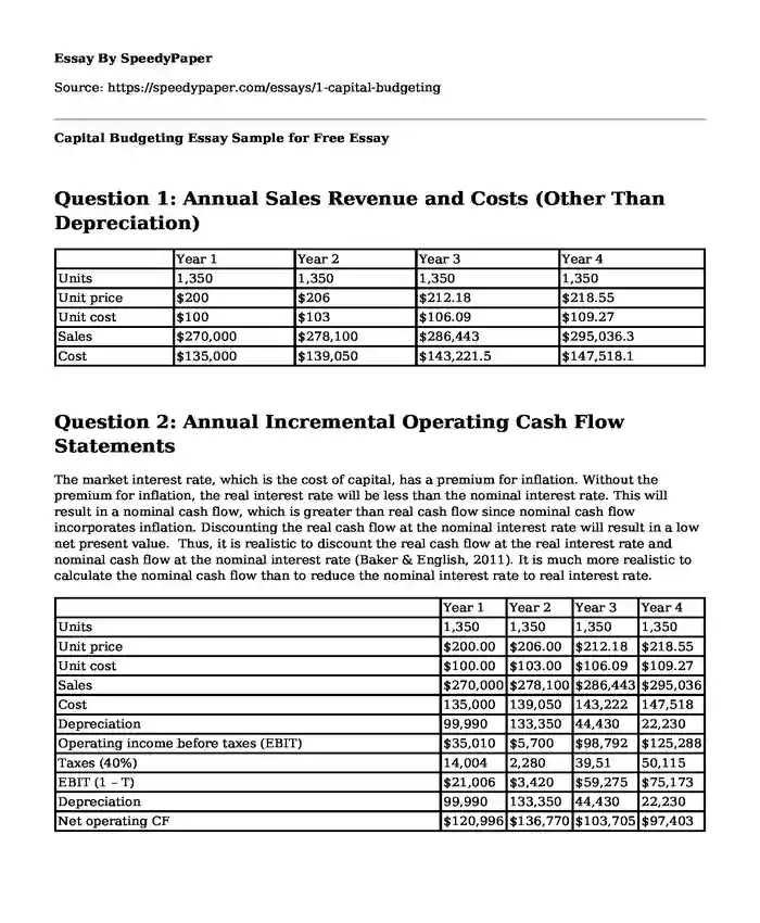
Question 1: Annual Sales Revenue and Costs (Other Than Depreciation)
| Year 1 | Year 2 | Year 3 | Year 4 | |
| Units | 1,350 | 1,350 | 1,350 | 1,350 |
| Unit price | $200 | $206 | $212.18 | $218.55 |
| Unit cost | $100 | $103 | $106.09 | $109.27 |
| Sales | $270,000 | $278,100 | $286,443 | $295,036.3 |
| Cost | $135,000 | $139,050 | $143,221.5 | $147,518.1 |
Question 2: Annual Incremental Operating Cash Flow Statements
The market interest rate, which is the cost of capital, has a premium for inflation. Without the premium for inflation, the real interest rate will be less than the nominal interest rate. This will result in a nominal cash flow, which is greater than real cash flow since nominal cash flow incorporates inflation. Discounting the real cash flow at the nominal interest rate will result in a low net present value. Thus, it is realistic to discount the real cash flow at the real interest rate and nominal cash flow at the nominal interest rate (Baker & English, 2011). It is much more realistic to calculate the nominal cash flow than to reduce the nominal interest rate to real interest rate.

| Year 1 | Year 2 | Year 3 | Year 4 | |
| Units | 1,350 | 1,350 | 1,350 | 1,350 |
| Unit price | $200.00 | $206.00 | $212.18 | $218.55 |
| Unit cost | $100.00 | $103.00 | $106.09 | $109.27 |
| Sales | $270,000 | $278,100 | $286,443 | $295,036 |
| Cost | 135,000 | 139,050 | 143,222 | 147,518 |
| Depreciation | 99,990 | 133,350 | 44,430 | 22,230 |
| Operating income before taxes (EBIT) | $35,010 | $5,700 | $98,792 | $125,288 |
| Taxes (40%) | 14,004 | 2,280 | 39,51 | 50,115 |
| EBIT (1 – T) | $21,006 | $3,420 | $59,275 | $75,173 |
| Depreciation | 99,990 | 133,350 | 44,430 | 22,230 |
| Net operating CF | $120,996 | $136,770 | $103,705 | $97,403 |
Annual Cash Flows Due To Investments in Net Working Capital
| Year 0 | Year 1 | Year 2 | Year 3 | Year 4 | |
| Sales | - | $270,000 | $278,100 | $286,443 | $295,036 |
| NWC (40% of sales) | 40,500 | 41,715 | 42,966 | 44,255 | - |
| CF due to investment in NWC | (40,500) | (1,215) | (1,251) | (1,289) | 44,255 |
After-Tax Salvage Cash Flow
| Salvage value | $25,000 |
| Book value | 0 |
| Gain or loss | $25,000 |
| Tax on salvage value (at 40%) | $10,000 |
| Net terminal cash flow | $15,000 |
Question 3: Projected Net Cash Flows
| Year 0 | Year 1 | Year 2 | Year 3 | Year 4 | |
| Long Term Assets | ($300,000) | 0 | 0 | 0 | 0 |
| Operating Cash Flows | 0 | $120,996 | $136,770 | $103,705 | $97,403 |
| CF due to investment in NWC | (40,500) | (1,215) | (1,251) | (1,289) | 44,255 |
| Salvage Cash Flows | 0 | 0 | 0 | 0 | 15,000 |
| Net Cash Flows | ($340,500) | $119,781 | $135,519 | $102,416 | $156,658 |
NPV = ∑ {Net Period Cash Flow/ (1+Rate) ^Time} - Initial Investment
= ($119,781/(1+0.12)1 )+($135,519/(1+0.12)2 )+($102416/(1+0.12)3)+($156,658/(1+0.12)4)-$300,000
= $46,939
IRR
IRR is the interest rate at which the net present value is equal to zero
IRR = 18.2%.
MIRR = (FVCF(c) / PVCF (fc)) ^ (1 / n) -1
= 15.7 %
PI
PI=Present value of future cash flows/Initial investment
= ($46,939+$ 300,000)/300,000
= 1.16
Payback Period
| Year | 0 | 1 | 2 | 3 | 4 |
| Cash Flow | ($340,500) | $119,781 | $135,519 | $102,416 | $156,658 |
| Cumulative Cash Flow for Payback | ($340,500) | ($220,719) | ($85,200) | $17,216 | $173,874 |
Payback Period= 2.8 Years
Discounted Payback Period
| Year | 0 | 1 | 2 | 3 | 4 |
| PV(CF) | 340500 | 106947.3 | 108034.9 | 72897.61468 | 99558.92 |
| Cash Flow for Payback | 340500 | -233553 | -125518 | -52620.1468 | 46938.77 |
Discounted payback period= 3.5 Years
The net present value rule indicates that a project is acceptable if the NPV is positive. In this case, the NPV is positive. The IRR rule, on the other hand, considers the value of IRR and the WAC. If IRR exceeds the WAC, then the project should be undertaken. IRR in this scenario is 18.2%, and WAC is 12%. Thus, the IRR exceeds WAC, and the project is fit to be undertaken. The MIRR rule is similar to that of IRR. Since MIRR is greater than the cost of capital, the project is accepted (Baker & English, 2011). The profitability index is 1.16, which, is higher than 1 meaning the project is profitable. The discounted payback period is 3.5 years. Both the payback period and the discounted payback period are less than the economic life of the machinery. The project will have paid back in 2.8 years and a discounted payback period of 3.5 while the economic life of the machine is four years. This indicates that the project is profitable and thus acceptable. All the rules of capital budgeting indicate that this project should be accepted.
Question 4: Risk
In the context of capital budgeting, a risk is a possibility of an investments actual returns being lower than the expected return. Risk involves losing some of the investment or the entire investment. The standard deviation measures the risk of specific investment or the average returns of the historical returns (Rüschendorf, 2013). A high standard deviation is a sign of a high degree of risk. Risk quantification occurs through attaching some probabilities to the happenings of negative events. If it is certain that, an event cannot occur, it gets a probability of zero, and if certain it will occur, it gets a probability of one. The probabilities of and only occur when the risk is certain. When the risk is uncertain, the probability assigned is between 0and 1. Maximum risk occurs when there is maximum uncertainty at the probability of 0.5.
Some types of project, historical data is very significant in assessing risk. The use of historical data is common when the investment involves an expansion. A company looking to expand can use its historical data to assess the risk involved. For a new business, a company can look at the historical data of other companies in the same line of business and assess risk. In some instances, historical data may not be available. In such a case, a company will have to depend on the judgment of the executives. Besides, some of the statistics used in analyzing historical data have its basis on subjective judgment. The availability of data determines the method used to quantify risk.
Question 5: Sensitivity Analysis
Sensitivity analysis is a technique used to determine how different values of an independent variable impact on a dependent variable under some given assumptions. It is a way of predicting the outcome of a decision made given a range of variables. It shows how a change in one variable affects the outcome. Capital budgeting incorporates sensitivity analysis to unearth the possible relationships between a project and profitability, sales, liquidity and the overall capital management of the entity.
- A) Primary Weaknesses
Among the major weaknesses of sensitivity analysis is that it is irrelative in nature. It only considers the extent of a change and not the probability of that change occurring. In addition, in standalone form, it offers no solution. The information it provides requires further analysis and interpretation to reach a decision (Baker & English, 2011). It also assumes that variables can change independently of other variables.
- B) Primary Usefulness
Sensitivity analysis is very simple and is a source of information to direct the managements’ planning efforts. Through its application, information becomes available to the management in a form that guides professional decision-making. In addition, it identifies areas where the management needs to concentrate in to attain the overall goal of the organization. The technique is significant in checking for quality (Baker & English, 2011). When the management know which variables are crucial to the success of a project, then they can b able to intensify the success of the project.
Sensitivity Analysis Diagram
| Deviation from | NPV Deviation from Base Case | ||
| Base Case | WACC (r) | Units Sold |
Salvage |
| -30% | $173,928 | $14,687 | $125,079 |
| -15% | 159,237 | 59,392 | 126,509 |
| 0% | 145,337 | 104,096 | 127,939 |
| 15% | 132,172 | 148,801 | 129,369 |
| 30% | 119,693 | 193,505 | 130,799 |
| Range | $54,235 | $208,193 | $5,720 |
A steep sensitivity line shows a greater risk. Along the line, a small change in any variables results to a decline in the net present value. From the graph above, the units sold line is steep than the interest rate and salvage value lines. This shows that a small change in estimated sales leads to a large decline in the net present value.. At the base case, the units sold are 104,096. A small change to the best or worst case yields a large margin in the change of number of units sold. If there are misestimates in the estimations of the sales and prices figures, then the net present value will differ by a great margin.
Cite this page
Capital Budgeting Essay Sample for Free. (2017, Nov 09). Retrieved from https://speedypaper.net/essays/1-capital-budgeting
Request Removal
If you are the original author of this essay and no longer wish to have it published on the SpeedyPaper website, please click below to request its removal:
- Reproductive system
- Essay Sample on Marketing and Sales Plan
- Peace, Propaganda and the Promised Land - Free Essay with Documentaries Analysis
- Officer in the U.S. Army, Essay Example for Students
- Essay Example: Frankenstein Critical Analysis Evaluation
- Stress and Stress Management - Research Paper Example
- Fulop, M. T., & Pintea, M. O. (2014). Effects of the new regulation and corporate governance of the audit profession. SEA-Practical Application of Science, 2(3), 5. HYPERLINK "https://econpapers.repec.org/RePEc:kap:jbuset:v:114:y:2013:i:3:p:457-471"
Popular categories