| Type of paper: | Essay |
| Categories: | Company Statistics |
| Pages: | 9 |
| Wordcount: | 2439 words |
Task 1: Summarising Data

Demographics
The company has 474 employees composed of 216 males and 258 females. The average salary paid by the company is £5441.36. The highest-earning employee is paid £25876.91, while the lowest earner in the company takes £2304.25. The income disparity between the lower earner and the highest earner is £23037.04. On average, most employees earn £4787.21. The average age of most employees is 37.186 years and the oldest person is 64.50 Years while the youngest person in the company is 23 years old. Most of the employees are 30 years. The mean salary now is13819.093 and the lowest salary now is £2807.42 while the highest salary now is £43896.31. Most people earn salaries above average.
Tem main issue facing the company include
1. Gender inequality. There are fewer women compared to men. For example, there are 216 female employees compared to 256 men.
2. Gender is also seen in incomes as the salary of some employee is relatively lower as compared to the salary of the male employees in the same position.
3. Most of the people in the higher position are men compared to only a few women.
4. Finally, the income or salary despite is also higher as the highest income earner takes home £54100 and the lowest salaried employees earn £2807.42. The range of the salary now is £41080.77.
5. The management need to understand the despite and sand implement solution aimed at ensuring that there equality in the company (Decker, Kipping, and Wadhwani, 2015).
There are trey variables.
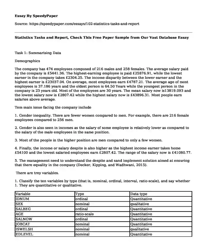
1. Classify the ten variables by type (that is, nominal, ordinal, interval, ratio-scale), and say whether 1. They are quantitative or qualitative.
| Variable | Type | Data type |
| IDNUM | ordinal | Quantitative |
| SEX | nominal | qualitative |
| SALBEG | ordinal | Quantitative |
| AGE | ratio-scale | Quantitative |
| SALNOW | ordinal | Quantitative |
| JOBCAT | nominal | Quantitative |
| ISWELSH | nominal | qualitative |
| EDLEVEL | nominal | Quantitative |
| AGEBAND | interval | Quantitative |
| SALNBAND | interval | Quantitative |
2. Using Excel, present the Job Category as a Pie Chart and as a Simple Bar Chart. Pay attention to labels, titles, and general neatness
3. Using Excel, use sensible grouping to organize the Salbeg data into a grouped frequency distribution and cumulative frequency distribution.
4. Using Excel construct a Histogram, Frequency Polygon and a Relative Cumulative Frequency curve for the data obtained in Q3 (the variable Salbeg). Pay particular attention to scale, labels, titles and general neatness.
| Anderson-Darling | Non-Normal at 0.01 |
| A-Squared | 8.202 |
| 0.000 | |
| 95% Critical Value | 0.787 |
| 99% Critical Value | 1.092 |
| Mean | 6544.084 |
| Mode | 5900.000 |
| Standard Deviation | 2719.522 |
| Variance | 7395798.801 |
| Skewedness | 2.296 |
| Kurtosis | 5.862 |
| 95.000 | |
| Std Err | 279.017 |
| Minimum | 3980.000 |
| 1st Quartile | 5000.000 |
| Median | 5900.000 |
| 3rd Quartile | 6500.000 |
| Maximum | 18896.000 |
| Range | 14916.000 |
| Confidence Interval | 553.995 |
6. By putting lines on the Relative Cumulative Frequency Curve estimate the median and quartiles of Salbeg. (can draw the lines using ‘Insert>Shapes>Lines' tool or handdraw them and scan the sheet in with your submission) What are the estimated values?
| Minimum | 3980.000 |
| 1st Quartile | 5000.000 |
| Median | 5900.000 |
| 3rd Quartile | 6500.000 |
| Maximum | 18896.000 |
| Range | 14916.000 |
6. Is the variable Salbeg symmetrical, negatively skew or positively skew? Write a short note summarizing the evidence for your answer.
The variable is positively skewed. The Skewedness is 2.296 positively skewed meaning that the symmetry of the probability distribution of the variables about the mean is positive. In this case, the model is significantly smaller than the median which is also much less than the sample mean. The data is normally distributed, and the longer tail is on the positive side to the graph peak or skewed or heavy to the right (Eriksson and Kovalainen, 2008).
Task 2: Regression & Correlation
1. Use Excel to obtain scatter plots and coefficients of correlation (r values please – not R2) for the following pairs of variables:
(a) Salary Now and Age.
R=0.145. The R values indicate that the model does explain all the variability of the response data around its mean.
SUMMARY OUTPUT Force Constant to Zero
FALSE
Regression Statistics
Multiple R0.145
R Square0.021Goodness of Fit < 0.80
Adjusted R Square0.019
Standard Error6753.012
Observations474
ANOVA
dfSSMSFP-value
Regression14610194610110.100.002
Residual4722152445603
Total 473 21985 Confidence Level
0.950.99
Coefficients Standard Error t Stat P-value Lower 95% Upper 95% Lower 99% Upper 99%
Intercept 16933.66 1027.505834 16.48035721 0.000 14914.61155 18952.71481 14276.24 19591.09
AGE -83.76 26.34236445 -3.179525414 0.002 -135.5190317 -31.99340273 -151.885 -15.6273
y = 16933.663 -83.756*AGE
RESIDUAL OUTPUTPROBABILITY OUTPUT
(b) Salary at Beginning and Age.
R=0.006. The value of R indicates that the model does not explain all the variability of the response data around the mean.
SUMMARY OUTPUTForce Constant to Zero
FALSE
Regression Statistics
Multiple R0.006
R Square0.000Goodness of Fit < 0.80
Adjusted R Square-0.002
Standard Error11.799
Observations474
ANOVA
dfSSMSFP-value
Regression12.52032.5200.018100.893
Residual47265715.6139.2
Total 473 65718.18 Confidence Level
0.950.99
Coefficients Standard Error t Stat P-value Lower 95% Upper 95% Lower 99% Upper 99%
Intercept 37.34235205 1.28132046 29.1436 0.000 34.8245 39.860 34.02 40.65
SALBEG -2.32938E-05 0.000173132 -0.13454 0.893 -0.00036 0.0003 -0.00047 0.0004
y = 37.342 0*SALBEG
(c) Salary Now and Salary at Beginning.
R=0.870. The value of R indicates that the model explains all the variability of the response data around its mean. Which means that the salary at the beginning is a good predictor of the salary now?
SUMMARY OUTPUTForce Constant to Zero
FALSE
Regression Statistics
Multiple R0.870
R Square0.757Goodness of Fit < 0.80
Adjusted R Square0.75
Standard Error3364.85
Observations474
ANOVA
dfSSMSFP-value
Regression116641625972166416259721469.8191410.000
Residual472534409114511322227
Total 473 21985717118 Confidence Level
0.950.99
Coefficients Standard Error t Stat P-value Lower 95% Upper 95% Lower 99% Upper 99%
Intercept 1125.406899 365.3930181 3.079990158 0.002 407.4086708 1843.405128 180.3962 2070.418
SALBEG 1.892827702 0.04937182 38.33822037 0.000 1.795811948 1.989843456 1.765138 2.020517
y = 1125.407 +1.893*SALBEG
RESIDUAL OUTPUTPROBABILITY OUTPUT
ObservationsPredictedSALNOWResidualsStandard ResidualsSorted ResidualsPercentileSALNOW
111157.39372-377.39372-0.11228###########0.105493460
210589.54541-1549.54541-0.46100###########0.316466400
Produce the results. Write a short note on what you think these graphs and r values tell you about the association between these variables.
From the association of the three variables. Age is not a good predictor of the salary now, and neither does it predicts the salary at the beginning. However, salary at the beginning can significantly predict the salary now (Bajpai, 2011). Which mean that if the entry salary of an individual is higher, then their salary now will be higher and if their beginning salary is low, then their salary now would be significantly low. Additionally, there are many other factors that may also inherently contribute in the value of salary including experience, age, employment category, educational level, and the ethnic background such as either one is welsh or not welsh. It is important to note that conducting a multivariate analysis can help in determining if among the many factors there are some that significantly predictor the independent variable (Balsley, Clover, and Clover, 1988).
2. Use Excel to calculate the regression equation of Salary Now on Salary at Beginning and to draw the line of this equation through the scatter plot.
Write out the equation in full.
For someone who began with a salary of 20,000, what would your regression line predict they would earn now? Would you have much faith in the accuracy of this forecast? Briefly, explain your answer.
y = 1125.407 +1.893*SALBEG
Salary Now=1124.407+ (1.893X salary at the beginning)
Foe someone who started with a salary of only 20,000, their salary now would be:
Y=1125.407+ (20,000X1.893)
Y=1125.407+37860
Y=38985.407
The salary now for the individual would be38985.407. From the equation, it is clear that the beginning salary is a good predictor of the salary now. However, the accuracy of the forecast is not 100% as there are a number of other factors that can influence the salary now apart from beginning salary. For example, professional level of education, task or nature of the job and other economic factors. However, in the absence of these extraneous factors, the beginning salary is a good predictor or salary now (Chesneau, 2007). Beginning salary significantly be predicted the salary now at F (1, 472) = 1469.819141, p<0.000 with an R2 of0.757. Beginning salary also explained a significant proportion of variance in salary now (Clover and Balsley, 1979).
Task 3: Probability
1. Use Excel to construct a pivot table (two-way table) of Sex and Educational Level. Submit this table. Then submit the table as if it was to be included in a page of a report: that is it must be completely self-explanatory with titles etc.
Row LabelsSum of SEX
030
1128
233
324
41
50
Grand Total216
2. If a member of staff is selected at random, what is the probability that they are:
(a) In the Professional Qualification category.
4%
(b) In the No Formal Qualification category.
11%
(c) Female.
67.90%
Row Labels Sum of the EDLEVEL
067.90%
132.10%
Grand Total100.00%
(d) Male.
32.10%
(e) In the Professional Qualification category given that they are female.
P (professional qualification) and probability (female)
=422/100x6790/100
=Probability that event A and event B occurs, P (A∪B): 0.692482
(f) In the Professional Qualification category given that they are male.
P(A∩B): 0.01344
(g) In the No Formal Qualification given that they are female.
0.07579872
(h) In the No Formal Qualification category given that they are male.
0.035712
3.Is Educational Level independent of Sex in this company? Explain your answer.
Education level is dependence on sex in the company. Most of the professional qualification workers are highly educated and are mostly men compared to the women. This means that most of the people in a position of power were men as compared to women while most women worked menial jobs in the company. This finding indicates the higher level of gender inequality that should be addressed by the top management. There may be possibilities that the management pony employs the most qualified person to the higher position and unfortunately, the women are not highly educated. As usual, correlation does not mean causality. Additionally, there is also significant income disparity as the range between the highest earners, and the lowers earner sis quite large. A range of $50,640 is too huge for a company. The income gap should be reduced by either increasing low-income earners salaries or reducing the salaries of the highest income earners.
Task 4: Probability Distributions
1. Which variables in the file are continuous?
Only AGE is continued variable
2. A new office, within the company, is to be established with eight occupants. Using the proportion of males to females in the company, and assuming an independent random selection of each office member with constant probabilities, draw up a probability distribution for the number of females in the office.
3. The Personnel Manager of the company has said: "salaries are fairly distributed in this firm over the whole salary range for both men and women, and we guarantee that (eventually) everyone will have a salary above 15,000".
Assume that by 'fairly distributed" the personnel manager means 'normally distributed.' Given this assumption, what would be the probability now of earning at least £12170.88 for males and females (separately)? What are the actual numbers (males and females) earning at least 1£12170.8? Does a comparison of these calculations support the personnel manager’s statement? Explain your answer.
The actual number of male and females that are likely to earn at least $15,000 is the difference as only 40% males, and 64 females are likely to earn more than $15000. The actual number of males and females that are likely to earn more than £12170.88 is 48% and 65% males and females respectively. The comparison of these calculations does not support those personnel’s manager’s statement because the relationship is not linear to be predictable. There are other extraneous factors that can influence the salary now of men and women. In ideal situation, the finding might come true as there are no other factors that might affect relationships and decision at work.
Reflection
The statistics and task report reveals that the company is considerably large with a significant number of employees who are well paid. Despite the development aspects achieved by the company, it has some challenges affecting its system, most of which influence the workers directly, for instance, the gender inequality issue. The use of the various statistical presentation methods makes the report easy to understand. For example, the use of pie chart, bar chart, histogram, and tables provides detailed information on a relatively small space. The histogram reveals that there is an impressive distribution of salaries among the men and women and there is a plan that soon everyone will have a net salary of more than a given figure. The Personnel Manager of the company on this note, reports that the salaries are fairly distributed in this firm over the whole salary range, and therefore will soon guarantee everyone to have a salary above £12170.88. It is, however, a challenge for the manager to prove that the implementation would mean a fair distribution of salary among the men and women owing to the fact that the relationship is not linear hence cannot be predicted. The number of males and females to earn above the mentioned figure does not support the argument given by the manager. The report confirms that the manager has failed to recognize some extraneous factors which may considerably influence the distribution and the subsequent increment of salaries for the men and women. There are other extraneous factors that can influence the salary now of men and women. However, it may turn out that the decision of the work may not be liable for the factors that negatively affect them, in which case, the situation may see the finding coming true due to the absence of such factors.
Bibliography
Bajpai, N. (2011). Business research methods. 1st ed. Delhi: Pearson.
Balsley, H., Clover, V. and Clover, V. (1988). Research for business decisions. 1st ed. Columbus, Ohio: Publishing Horizons.
Chesneau, C. (2007). Regression with random design: A minimax study. Statistics & Probability Letters, 77(1), pp.40-53.
Clover, V. and Balsley, H. (1979). Business research methods. 1st ed. Columbus, Ohio: Grid Pub.
Decker, S., Kipping, M. and Wadhwani, R. (2015). New business histories! Plurality in business history research methods. Business History, 57(1), pp.30-40.
Eriksson, P. and Kovalainen, A. (2008). Qualitative methods in business research. 1st ed. Los Angeles: SAGE.
Eryilmaz, S. (2011). Joint distribution of run statistics in partially exchangeable processes. Statistics & Probability Letters, 81(1), pp.163-168.
Feller, W. (1957). An introduction to probability theory and its applications. 1st ed. New York: John Wiley & Sons, Inc.
Feller, W. (1957). An introduction to probability theory and its applications. 1st ed. New York: John Wiley & Sons, Inc.
Fuller, C., Simmering, M., Atinc, G., Atinc, Y. and Babin, B. (2016). Common methods variance detection in business research. Journal of Business Research, 69(8), pp.3192-3198.
Harrison, R. (2013). Using mixed methods designs in the Journal of Business Research, 1990–2010. Journal of Business Research, 66(11), pp.2153-2162.
Krishnaswamy, O. and Satyaprasad, B. (2010). Business research methods. 1st ed. Mumbai [India]: Himalaya Pub. House.
Marcoulides, G. (1998). Modern methods for business research. 1st ed. Mahwah, N.J.: Lawrence Erlbaum.
Oppewal, H., Louviere, J. and Timmermans, H. (2000). Modifying Conjoint Methods to Model Managers' Reactions to Business Environmental Trends. Journal of Business Research, 50(3), pp.245-257.
Saunders, M., Lewis, P. and Thornhill, A. (2007). Research methods for business students. 1st ed. Harlow, England: Financial Times/Prentice Hall.
Zikmund, W. (2003). Business research methods. 1st ed. Mason, OH: Thomson/South-Western.
Cite this page
Statistics Tasks and Report, Check This Free Paper Sample from Our Vast Database. (2018, Feb 07). Retrieved from https://speedypaper.net/essays/102-statistics-tasks-and-report
Request Removal
If you are the original author of this essay and no longer wish to have it published on the SpeedyPaper website, please click below to request its removal:
- Louis Armstrong Essay Samples
- Fire Prevention Essay Sample
- Essay Sample: Impact of Social and Personal Factors
- Free Essay: PepsiCo Company Overview and Porter's Five Forces Analysis
- Job Satisfaction - Articles Review Paper Sample
- Creative Writing Essay Example on Images as Inspiration: The Skat Players
- DateHomer's The Odyssey Book 12
Popular categories